One of many comparisons between countries is the size of their economies. In the recent past, a number of people noted that Nigeria had overtaken South Africa as the largest economy on the African continent. Subsequently, articles were written about South Africa being pushed into third place by Egypt, only to regain the silver medal position shortly thereafter.
We live in a relative world, in which comparisons are ever-present. Which car is faster? Who can jump higher or further? Which shop is cheaper? Who is the better dancer or bowler or painter? Many comparisons can be put to the test using a stopwatch or measuring tape or simple counting. Others are a matter of judgement.
So how accurate are comparisons of economic size? We must ensure that we are comparing similar measurements of the economy. This means that all countries being compared must follow the same accounting conventions and standards. When measuring the economy, these estimates should be guided by the System of National Accounts. Many countries follow the 1993 version of the framework (regrettably a number of countries still follow the 1968 version of the SNA), whereas some have implemented the latest 2008 set of recommendations. The move from 93SNA to 08SNA often requires substantial revisions, as new definitions and concepts are included in the measurement of the economy. In the South African case, it is estimated that the move between accounting systems added 1,2% to the size of the economy.
Price, quantity and value
Once we are sure that we are using the same accounting method and we trust that the quality of the data is good, we need to be careful that we compare the correct values. The size of the economy is calculated through estimates of gross domestic product (GDP). Since GDP represents the value (V) of all goods and services produced in a country during a specific period, it is a function of the quantity (Q) of goods and services as well as the price (P) of goods and services. Typically economists go to great lengths to remove the impact of changes in P from the GDP estimates, thereby expressing them in ‘real’ or ‘volume’ terms. This makes it possible to calculate economic growth rates based on changes in Q. For example, suppose a firm produces 100 shirts (Q) and sells them for R150 each (P). V = PQ = (100)(R150) = R15 000. If Q increases to 110 and P increases to R180, V = (110)(R180) = R19 800. The percentage change in V is 32%. But if we’re interested in the change in V in real terms (no price effect), the new V is (110)(R150) = R16 500. Now the percentage change in V is 10%, which is identical to the percentage change in Q.
Converting GDP from SA rands to US dollars
For the purpose of comparing the size of GDP between countries, we need to take a different approach. In the equation V = PQ each country expresses the price of the goods and services in its own currency. But this makes comparisons between countries futile. We need to express the value in comparable terms, which requires that in V = PQ, P must be the same unit of measurement. This is often done by converting each country’s local currency P to a United States dollar (US$) P, using the prevailing exchange rate. Figure 1 shows how this can be calculated for South Africa by using the R/$ exchange rate to express nominal GDP in US$ terms.
Figure 1
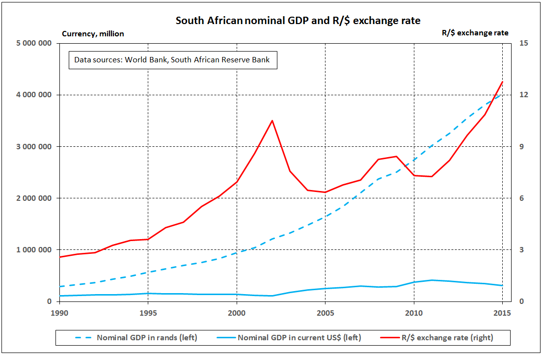
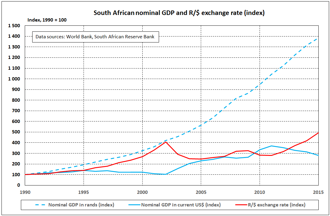
Figure 2
In 1990 South Africa’s GDP was estimated at R290 billion, and with an exchange rate of R2,59/$, the economy was worth $112 billion. In 2002 the exchange rate depreciated significantly to R10,52/$, so GDP of R1 217 billion became $115 billion. And for 2015, a R4 014 billion economy translates to a $315 billion economy.
The picture becomes more clear if we index the values to 1990 = 100 as shown in Figure 2. Nominal GDP grows from the base of 100 in 1990 to 420 in 2002 and 1 385 in 2015. But in US$ values, the index grows to only 103 and 281 in the corresponding years. This is because the indexed exchange rate moved to 406 (2002) and 493 (2015). The choice of currency, therefore, tells a different story about the behaviour of the economy. In some instances, the R/$ changes, but nothing has really changed that much in the actual economy. We can use the period 2002 – 2003 to illustrate this. In nominal rand terms, the economy expanded by 9%, which is an increase that mirrors what would anecdotally be expected. But in US$ terms, it expanded by 52%! This is purely because of the huge recovery in the exchange rate rather than any significant economic growth in the actual economy.
Purchasing power parity
Noting the pitfalls in describing the economy in a currency other than that of the country in question, the problem can be magnified when using a common currency to make cross-country comparisons. Extreme care must be taken to understand the behaviour of an economy measured in a foreign currency. A further shortcoming of the common currency approach, using actual exchange rates, is that comparisons of GDP fail to take price differences into account, i.e. if there are large price differences between countries (measured in the same currency), purchasing power differences are not considered. Consequently, an alternative way to compare GDPs is to use purchasing power parity exchange rates.
The World Bank provides the following definition: ‘Purchasing power parities (PPPs) are the rates of currency conversion that equalize the purchasing power of different currencies by eliminating the differences in price levels between countries. In their simplest form, PPPs are simply price relatives that show the ratio of the prices in national currencies of the same good or service in different countries. PPPs are also calculated for product groups and for each of the various levels of aggregation up to and including GDP.’ 1
For example, suppose an item costs R630 in South Africa and $90 in the United States. If the actual exchange rate is R9/$, a South African would need R810 to purchase the item in the United States (the South African’s purchasing power has declined). For the South African to purchase the same item in the United States for R630, the exchange rate would have to be R7/$ – and this is known as the purchasing power parity (PPP) exchange rate. Measured at the actual exchange rate of R9/$, the value of the item in South Africa would be $70 (630/9). Measured at the PPP exchange rate of R7/$, the value of the item in South Africa would be $90 (630/7). In this case, where it is expensive for South Africans to go shopping in the United States, use of the actual exchange rate undervalues the item (in US dollars) in South Africa, which is where South Africans usually shop. Of course, the calculation of PPP exchange rates is vastly more complex than this simple example, since there are so many goods and services to consider.
The World Bank calculates PPPs for each country in terms of the US dollar. For example, in 2015 the PPP R/$ exchange rate was 5,53 (whereas the actual R/$ rate was 12,75). The PPP$ is linked to the US$ for practical purposes and is based on extensive projects that are commissioned periodically. The latest of these international comparison projects (ICPs) were done in 2005 and 2011. These projects rely on participating countries to provide detailed data on the expenditure on GDP by the various components on different goods and services as well as detailed prices for a common basket of goods and services. In many cases, countries had to specially collect prices for goods and services that would not ordinarily be included in their consumer price index basket. By combining detailed expenditure weights with corresponding prices, it is possible to derive estimates of PPP$s for each country. Using PPP$s allows for the comparison of economies with the advantage of a common “P” but without the pitfalls of volatile exchange rate fluctuations.
Country comparisons using the US dollar
In Figure 3 the changes in size over time of the economies of South Africa, Nigeria and Egypt are shown using a direct conversion from the local currency into US$ at the prevailing market rate.
Figure 3
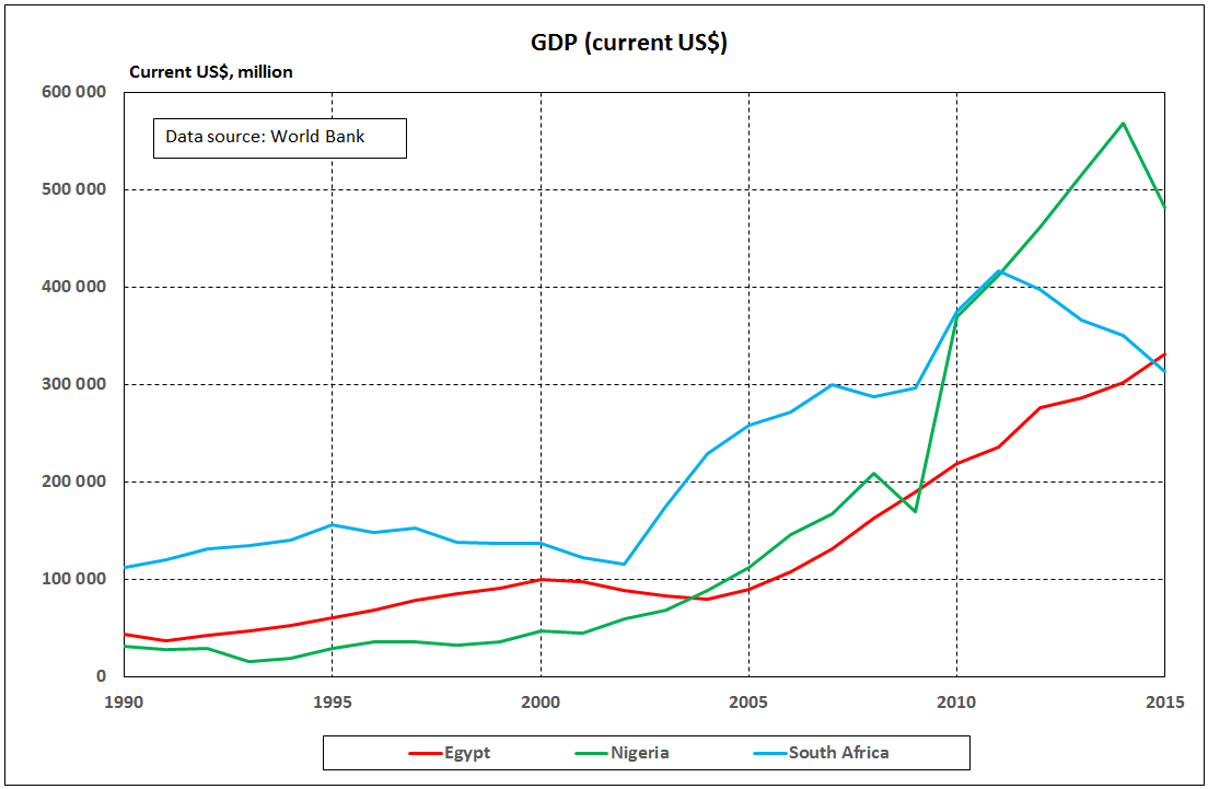
In 1990, the US$ equivalents of the economies were as follows: Nigeria $31 billion, Egypt $43 billion, and South Africa $112 billion. The graph shows how the Egyptian economy grew strongly in the 1990s, while South Africa declined in the latter half of the decade. The Nigerian economy expanded from $32 billion in 1998 to $208 billion in the next 10 years. In 2009, Nigeria had a dip of 19% (global economic crisis), but the following year saw a sharp upward spike of 118%. On this measure of GDP, Egypt had positive growth every year from 2005, while South Africa had positive growth most years between 2003 and 2011, but negative growth thereafter.
But how much of this growth was due to exchange rate changes rather than changes in the actual economy?
Country comparisons using purchasing power parity
In Figure 4 the nominal size of the three economies are expressed in PPP$. In 1990, South Africa had the largest economy (PPP$236 billion), followed by Egypt (PPP$219 billion) and Nigeria (PPP$187 billion). In 1992, Egypt became larger than South Africa and this ranking held until 2004 when Nigeria moved into second place. In 2011, Nigeria overtook Egypt in the rankings as the largest economy of the three countries.
Figure 4

The stories in Figures 3 and 4 are vastly different. Figure 4 is more accurate, as it uses a conversion to a common currency that is based on actual prices and expenditure information in the countries, rather than market exchange rates that can be volatile and influenced by many factors. The movements in the PPP$ graph are consequently also more gradual, which is just as expected.
Data revisions and quality
Unfortunately, it is never quite as simple as this. As part of international best practice, countries will periodically make revisions to their official statistics. There are various reasons for revisions, but two main reasons dominate. First, new data become available that provide more accurate estimates of economic behaviour. This could include periodic population censuses, household expenditure surveys, comprehensive surveys of businesses, as well as new surveys designed to measure economic phenomena that were not previously recorded. Second, revisions are done when methodological changes are introduced, e.g. moving from 93SNA to 08SNA or a change in the use of a classification standard.
Table 1 compares the US$ size of the three economies based on official data that were submitted as part of the 2011 ICP round with the latest estimates as used above (i.e. Figure 3). Given that the actual market exchange rates cannot be revised, any revision is due to revisions in the estimates of the economy by the country. The well-documented upward revision of the size of the Nigerian economy is clearly evident in the statistics.
Revisions should be explained in a transparent manner to the user community, and they should not be unexpected. Communication and transparency are key to building trust in official statistics.
Table 1: Size of economy (US$ billion) in 2011
Country
|
2011 ICP estimate
|
Latest estimate for 2011
(as shown in Fig. 3)
|
Percentage revision
|
| Egypt |
229
|
236
|
3
|
| Nigeria |
247
|
412
|
67
|
| South Africa |
401
|
416
|
4
|
Although countries may follow the same version of the SNA, the quality of their estimates of national accounts could be different. Some may not include all aspects of economic activity, or may not have access to regular statistical surveys that underpin reliable measures of the economy. These differences in scope and coverage in national accounts are complex and can be difficult and expensive to quantify. Using the same unit of measure goes a long way towards making comparisons easier, but care should be exercised as to what this common measure is.
Reference:
1. http://www.statssa.gov.za/?p=9583